|
|
|
|

courtesy of C. Kerfeld. |
Isomorphous Differences:
A sample
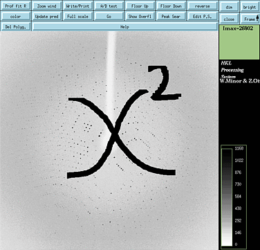
script for the isomorphous Chi Squared test is given below. You need
a complete native data set in scalepack format (.sca file) and only 5 degrees
of integrated data (.x files) from a derivative data set. Since you
can perform this test after only 5 frames, it can be used to quickly decide whether
to collect a full data set or move on to the next putative derivative crystal.
If the chi squared statistics for your
crystal are
small
(under 3 in all resolution ranges) then you can be guaranteed
that this crystal is not useful for phasing. It is essentially, a native
crystal. If the chi squared statistics for your crystal are large
then there is hope that you have a
useful derivative.
But remember, a positive result on the isomorphous chi squared test is
not always reliable since non specific heavy atom binding often causes
non-isomorphism
between native and derivative crystals ...which in turn
leads to large chi squared values. Alas, false positives are common. If
you have a positive isomorphous chi squared test, then you should continue
collecting data until over 90% complete. Then calculate an isomorphous
difference Patterson map to check for peaks on the Harker sections. Harker
peaks greater than 5 sigma are an indisputable indication of a useful derivative!
Example log files
from 1) a
good
derivative 2)
non-isomorphous
derivative
and 3)
non-derivative
are given below.
Manual for Denzo:
|
|
|
|
|
scalepack << eof-scale > scalepotder.log space group P61
format scalepack hkl matrix 1 0 0
file 1 'native.sca'
[**********Potential Derivative***********]
estimated error .05 .05 .05 .05 .05 .05 .05 .05
error scale factor 1.6 rejection probability 0.0001 ignore overloads add partials 1 to 6 format denzo_ip sector 1 to 6 hkl matrix 1 0 0
file 2 'deriv_1_###.x' output file 'junk.sca' eof-scale
|
We are licensed to use Scalepack on Sayre or Bayes.
First we specify space group and location of native data set. Check the native scalepack log file --the chi squared values given in
the last table of the log file should be close to 1.0 in all resolution
shells. If not, run another cycle of scalepack on the native data set,
adjusting the estimated error estimates until chi squared is between 0.9
and 1.1. The error estimates used in the native data set will effect the
chi squared test when comparing with the derivative.
Here we specify information about the derivative crystal.
add partials. We are using frames 1-6 in this example.
|
|
|
| Here is an example log file for a true Hg derivative of
a 30kD protein (T7 helicase domain in space group P61). Notice that the
Rfactor for useful data is between 10% and 30%. Any less than 10% and the
derivative is probably really a native. Also Chi squared should be somewhere
between 2 to 50. The isomorphous difference Patterson map showed 8 sigma
peaks on the harker sections.
Summary of reflections intensities and R-factors by shells
Shell Lower Upper Average Average
Norm. Linear Square
|
|
|
| Here is an example log file from a non-isomorphous derivative
(Courtesy of C. Goulding).
Heavy atoms bind non-specifically and cause changes in crystal packing.
The result is large differences in the chi squared test which closely mimic
the results from the chi squared test from an true isomorphous derivative
(see above). When you get a result like this, you need to continue collecting
data until the data set is better than 90% complete. Then calculate an
isomorphous difference Patterson map. In this example, the Patterson map
was flat on all the harker sections.
Lower Upper Average Average. Norm. Linear Square I error stat. Chi**2 R-fac R-fac 99.00 7.00 1784.6 47.8 37.0 170.026 0.196 0.356 7.00 5.56 1391.3 34.3 30.2 19.617 0.172 0.230 5.56 4.85 2089.4 42.8 37.4 50.743 0.201 0.423 4.85 4.41 1975.4 35.7 32.0 84.048 0.253 0.451 4.41 4.09 1841.8 41.3 37.6 42.016 0.256 0.427 4.09 3.85 1434.4 36.8 36.3 37.648 0.268 0.580 3.85 3.66 1439.1 45.7 45.1 52.823 0.338 0.536 3.66 3.50 1361.5 53.7 53.4 53.058 0.447 0.745 All reflections 1671.8 42.4 38.5 69.212 0.232 0.422 |
|
|
| Here is an example log file for a non-derivative.
The chi squared test indicates no significant differences between the
native and derivative. In fact, it looks like the logfile you would
expect from scalepacking a single native crystal. When you get test
results like this, remove the crystal from data collection and try a
different soak condition.
Lower Upper Average Average
Norm. Linear Square
|