|
|
|
|
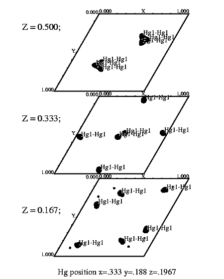
T7 helicase domain ethylmercurythiosalicylate derivative. Spg P61. |
The Isomorphous Difference Patterson
map is simple to calculate with the XtalView suite of programs. The program
produces a contoured map, which may be displayed and re-contoured interactively
in sections along x, y, or z. There is a small investment in time to setup
to use XtalView (10 minutes). However, you only have to do it once. I have
constructed a web page to assist you in setting
up to use XtalView. Once you have setup, then follow the steps outlined
below for producing an isomorphous difference Patterson map.
Requirements:
Manual for XtalView:Manpages or User guide Reference for XtalView:
Reference for the Isomorphous difference Patterson
Map:
|
|
|
|
| If you are setup
to use XtalView, you may proceed as follows. If not, go here
.
STEP ONE Use xprepfin to convert your scalepack file for the native crystal (native.sca) to .fin format (native.fin). In a unix window, type: xprepfin native.sca native.fin Choose the buttons such that:
Then press the "Apply" button.
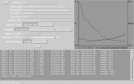
xprepfin hg.sca hg.fin STEP TWO Use xmerge to merge your native.fin and hg.fin files into a double fin file (e.g. isomorphous.df). In a unix window, type: xmerge native.fin hg.fin isomorphous.df Since we have plenty of reflections we can set the slider to 20 bins: Press "Single" meaning that a single scale factor will be used. You may also want to try "anisotropic" to get a better fit, but beware, sometimes this fails. Check the R-factors with xstat. In a unix window type: xstat isomorphous.df Select: R-factor vs. resolution
Then press the Graph It button. You will get two windows:
These windows will indicate if the scaling is correct and suggest a resolution range to use in the isomorphous difference Patterson map. STEP THREE In a unix window, type: xfft isomorphous.df isomorphous.map Choose the buttons such that:
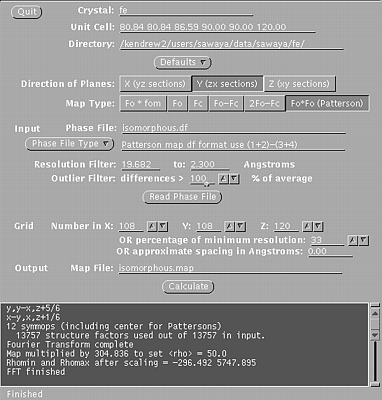
Type in your resolution range. Be sure to press Enter everytime you enter a new number. Press Read Phase File
Xfft will automatically select grid units appropriate
for your unit cell and resolution.
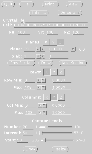
STEP FOUR Display map with xcontur. In a unix window type: xcontur isomorphous.map Press the "next" button to page through the sections of your map. Look for peaks over 5 sigma. The maps are automatically scaled so that a peak height of 50 is equal to 1 sigma. So look for peaks of height 250 (5 sigma). You can determine the peak height by simply clicking on the peak. Be sure to select x, y, and z limits that cover your asymmetric unit. If you want to see the whole unit cell, chose limits of 1.0 for rows and columns. In this example, the space group is P61, so there are three harker sections, (z=.166, z=.333, z=.500). The example window on the right, is set to view the Harker section at z=.333, a cross section through the unit cell. The map section should look like one of the sections in the image displayed at the top of this file. The contour levels start at 1 sigma and the intervals are set at one sigma. The highest peak on the Harker section is about 7 sigma (level 350). |
Xprepfin window, used in step one.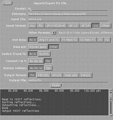
Xmerge window, used in step two.
Xfft window, used in step three.
Xcontur window, used in step four.
|
