An inversion is a symmetry operation which acts on every atom at coordinates $[x, y, z]$ to generate a symmetry-equivalent counterpart at coordinates $[-x, -y, -z]$. These atoms end up equidistant from a unique point called the center of inversion, which is usually defined as the origin. We generally refer to space groups containing these elements of symmetry as centrosymmetric. By definition, centrosymmetric space groups can only accommodate achiral assemblies of molecules, since enantiopure, homochiral molecules cannot undergo inversion and emerge unscathed. In terms of transformation matrices, an inversion is represented by the negated identity matrix, as follows: \begin{equation} \begin{bmatrix} -1 & 0 & 0 \\ 0 & -1 & 0 \\ 0 & 0 & -1 \end{bmatrix} \begin{bmatrix} x \\ y \\ z \end{bmatrix} = \begin{bmatrix} -x \\ -y \\ -z \end{bmatrix} \\ \end{equation} The simplest centrosymmetric space group, P$\bar{1}$, contains a single center of inversion (termed $\bar{1}$ in Hermann-Mauguin notation) as its only element of symmetry. Incorporating this into the structure-factor equation, we obtain \begin{equation} F_{hkl}=\sum_{j} f_{j}(s)\,\exp[2\pi i\,(hx_{j} + ky_{j} + lz_{j})]+f_{j}(s)\,\exp[2\pi i\,(-hx_{j} - ky_{j} - lz_{j})]. \end{equation} We can simplify this into a more suggestive form by removing a common factor of $-1$ from the second term, yielding \begin{equation} F_{hkl}=\sum_{j} f_{j}(s)\,\underbrace{\exp[2\pi i\,(hx_{j} + ky_{j} + lz_{j})]}_{\exp(i\phi)}+f_{j}(s)\,\underbrace{\exp[-2\pi i\,(hx_{j} + ky_{j} + lz_{j})]}_{\exp(-i\phi)}. \end{equation} What we're seeing here is a just a pair of glorified complex conjugates, which we can express more abstractly as $\exp(i \phi)$ and $\exp(-i \phi)$. This is simply a slightly convoluted case where $\phi = 2\pi (hx_{j} + ky_{j} + lz_{j})$. Recall that $\mathrm{exp}(i \phi)+\mathrm{exp}(-i \phi)=2\,\mathrm{cos}(\phi)$. This is a direct consequence of the fact that the cosine function is centrosymmetric, whereas the sine function isn't. In other words, in reciprocal space, we can fully describe the Fourier transform of the atomic charge density function in a P$\bar{1}$ unit cell using cosine waves alone. Summing complex conjugates, we get \begin{equation} F_{hkl}=2\sum_{j} f_{j}(s)\,\cos{[2\pi(hx_{j} + ky_{j} + lz_{j})]}. \end{equation} This expression conveys a key fact about $F_{hkl}$ in P$\bar{1}$: it's always real, which ultimately provides us with a powerful constraint on the permissible phases. Furthermore, thanks to Friedel's law, we also know that an arbitrary reflection [$hkl$] and its Friedel mate [$\bar{h}\bar{k}\bar{l}$] have the same structure-factor amplitudes \begin{equation} |F_{hkl}| = |F_{\bar{h}\bar{k}\bar{l}}| \end{equation} but opposite phases: \begin{equation} \phi_{hkl} = -\phi_{\bar{h}\bar{k}\bar{l}}. 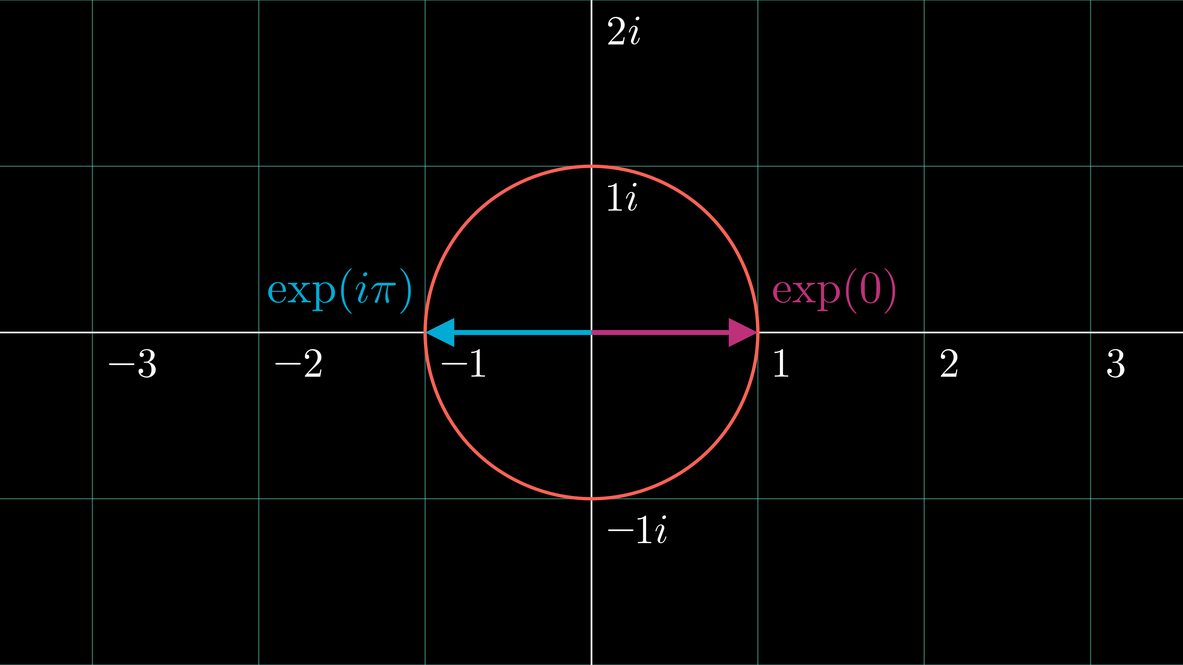\end{equation} Mathematically, precisely two scenarios exist which preserve these combined constraints. You guessed it: the only phases consistent with these restrictions are 0 and $\pi$! To explicitly substantiate this point, let's analyze it geometrically. We can conceptualize $F_{hkl}$ and $F_{\bar{h}\bar{k}\bar{l}}$ as two vectors in the complex plane. Friedel's law tells us that their magnitudes must be equal, so the two vectors remain confined to a unit circle with a fixed radius. For simplicity's sake, let's set the radius to $|F_{hkl}| = 1$, so now we're essentially just comparing $\exp(i\phi_{hkl})$ and $\exp(-i\phi_{\bar{h}\bar{k}\bar{l}})$. The vectors' position on that unit circle is governed by the value of $\phi$. However, Friedel's law also mandates that the phase of reflection [$hkl$] is equivalent to the negated phase of its Friedel mate [$\bar{h}\bar{k}\bar{l}$]. Now let's add the final constraint, which we derived earlier: $F_{hkl}$ must be real! This means we're looking for two values of $\phi$ which collapse $F_{hkl}$ to the real axis.¹ As expected, the only phases which satisfy these restrictions work out to be 0 and $\pi$, since $0 = -0$ and $\pi$ radians = $-\pi$ radians: \begin{equation} \exp(0) = \exp(-0) = 1 \end{equation} \begin{equation} \exp(i\pi) = \exp(-i\pi) = -1 \end{equation}

It's easy to show that any other argument for $\phi$ makes $\exp(i\phi_{hkl})$ and $\exp(-i\phi_{\bar{h}\bar{k}\bar{l}})$ complex numbers—thus violating the "keep it real" constraint we derived above. These relations also allow us to deduce the phase of any structure factor in a centrosymmetric space group simply by looking at its sign. If $F_{hkl}$ is positive, $\phi_{hkl}=0$; conversely, if $F_{hkl}$ is negative, $\phi_{hkl}=\pi$.

Now let's develop these ideas by taking what might initially seem like a counterintuitive step. Let's hunt for phase restrictions in a non-centrosymmetric space group: $\text{P}2_{1}$. $\text{P}2_{1}$ is one of the 65 Sohncke groups, indicating that its lack of inversion or mirror symmetry lets it accommodate homochiral, enantiopure molecules (like proteins). Recall that the structure-factor equation in P2$_{1}$ incorporates the symmetry operator $(-x, \tfrac{1}{2} + y, -z)$, yielding \begin{equation} F_{hkl}=\sum_{j} f_{j}(s)\{\exp[2\pi i\,(hx_{j} + ky_{j} + lz_{j})]+ \exp[2\pi i\,(-hx_{j} + k\{\tfrac{1}{2} + y_{j}\} - lz_{j})]\}. \end{equation} An eerily familiar result quickly emerges if we focus our attention on the $[h0l]$ set of reciprocal lattice points. Substituting $k=0$, we get \begin{equation} F_{h0l}=\sum_{j} f_{j}(s)\,\{\mathrm{exp}[2\pi i\,(hx_{j} + lz_{j})]+\mathrm{exp}[2\pi i\,(-hx_{j} - lz_{j})]\}. \end{equation} Factoring out $-1$ from the second term gives us \begin{equation} F_{h0l}=\sum_{j} f_{j}(s)\,\underbrace{\exp[2\pi i\,(hx_{j} + lz_{j})]}_{\exp(i\phi)}+f_{j}(s)\,\underbrace{\exp[-2\pi i\,(hx_{j} + lz_{j})]}_{\exp(-i\phi)}. \end{equation} Believe it or not, we've once again stumbled across a pair of complex conjugates. Summing these, we arrive at \begin{equation} F_{h0l}=2\sum_{j} f_{j}(s)\,\cos{[2\pi(hx_{j} + lz_{j})]}. \end{equation} Applying the same logic as before, we can surmise that $F_{h0l}$ in $\text{P}2_{1}$ must be real, which guides us to the conclusion that its phases are constrained to either 0 or $\pi$! Why, though, is this restriction materializing in what could easily appear like an arbitrary zone of the reciprocal lattice? In other words, what's so special about $[h0l]$? The answer is surprisingly straightforward: phase restrictions arise whenever our space group contains a symmetry operator whose rotational component inverts the Miller indices of a given structure factor (i.e., generates its Friedel mate). In $\text{P}2_{1}$, as we derived earlier, a $2_{1}$ screw axis parallel to the unit cell vector b generates the symmetry-equivalent position $(-x, \tfrac{1}{2} + y, -z)$. Clearly, the rotational component of this $2_{1}$ screw axis inverts the $x$ and $z$ coordinates. To obtain the corresponding symmetry operator in reciprocal space, we take the inverse² of its real-space counterpart and omit the translational component: \begin{equation} \textbf{R}^{-1}= \begin{bmatrix} -1 & 0 & 0 \\ 0 & 1 & 0 \\ 0 & 0 & -1 \end{bmatrix}^{-1} = \begin{bmatrix} -1 & 0 & 0 \\ 0 & 1 & 0 \\ 0 & 0 & -1 \end{bmatrix} \end{equation} which in this particular case just gives us the same operator, because the input matrix was orthogonal and symmetric.³ Applying this to $[h0l]$, we get \begin{equation} \begin{bmatrix} -1 & 0 & 0 \\ 0 & 1 & 0 \\ 0 & 0 & -1 \end{bmatrix} \underbrace{ \begin{bmatrix} h \\ 0 \\ l \end{bmatrix}}_{\textbf{h}} = \underbrace{ \begin{bmatrix} \bar{h} \\ 0 \\ \bar{l} \end{bmatrix}}_{\textbf{-h}} \end{equation} indicating a sort of local inversion symmetry confined to this region of the reciprocal lattice. These centric reflections occur whenever a pair of Bragg peaks is related not just by Friedel's law but also by the point-group symmetry of the crystal. Using the syntax of linear algebra, an elegant way to express this idea is as an eigenproblem: \begin{equation} \boxed{\textbf{R}^{-1} \, \textbf{h} = \lambda \, \textbf{h}} \end{equation} where $\textbf{R}^{-1}$ is the relevant reciprocal-space rotation matrix, $\textbf{h}$ is a column vector representing a set of Miller indices, and $\lambda = -1$. If $\textbf{h}$ is an eigenvector of $\textbf{R}^{-1}$ whose corresponding eigenvalue $\lambda$ is $-1$, $\textbf{R}^{-1}$ will always map $\textbf{h}$ to $-\textbf{h}$, fulfilling the criteria for centricity. Critically, in $\text{P}2_{1}$, this phase restriction only applies to a specific subset of reflections located in one particular zone of the reciprocal lattice (i.e., where $k = 0$). Some arbitrary reflection located anywhere else in reciprocal space remains unrestricted: it could legally exhibit any random phase angle, making it acentric. In algebraic terms, as long as some arbitrary set of Miller indices $\textbf{h}$ is not an eigenvector of $\textbf{R}^{-1}$, it's completely unaffected by phase constraints. Conversely, in an achiral, centrosymmetric space group like $\text{P}\bar{1}$, every single reflection is centric (i.e., globally subject to the $\phi_{hkl} = 0$ or $\pi$ constraint). This follows intuitively from the fact that $\textbf{R}^{-1} = -\textbf{I}$ in $\text{P}\bar{1}$, so every possible set of Miller indices $\textbf{h}$ is an acceptable solution to the eigenproblem.

What advantage does centrosymmetry provide for phase retrieval? Well, it drastically limits our choices. We're basically going from guessing any random angle between 0 and $2\pi$ to choosing between exactly two options. Furthermore, we're 100% confident that one of those two options must be correct. This greatly simplifies our search for the correct phases. Even so, if we measure $x$ unique reflections in our dataset, that means we have $2^{x}$ possible combinations of amplitudes and phases... which starts to look mildly quixotic if $x$ is something like 100000. That's why it always helps to have some external source of information (like the probabilistic relationships between phases originally derived by Hauptman and Karle) that empowers us to make better-than-random guesses.

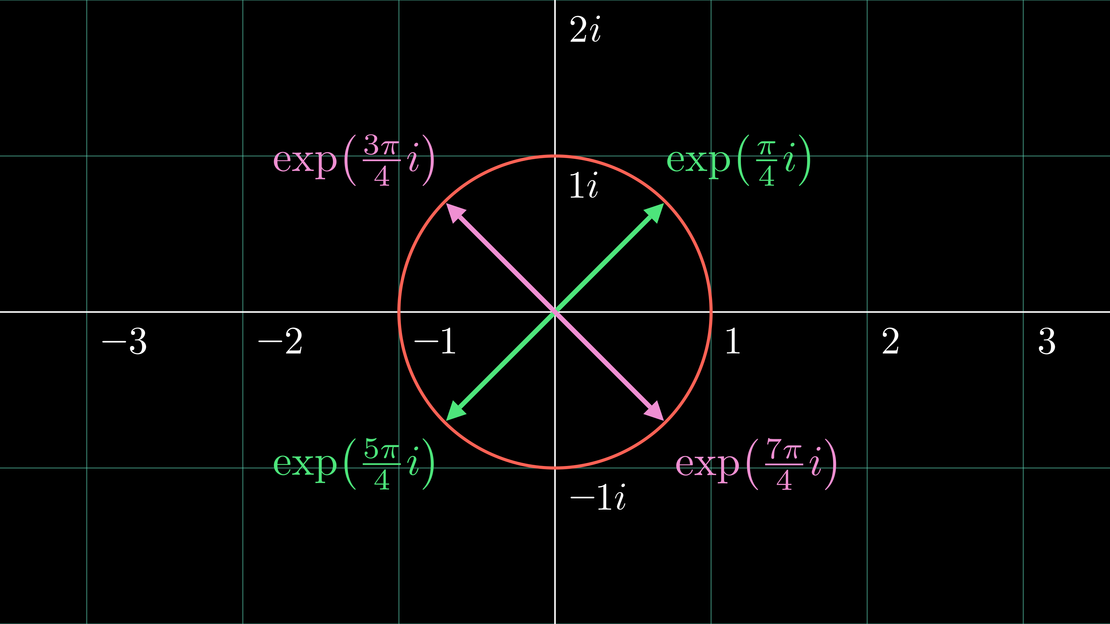
1. So far, we've only looked at phase restrictions arising from $F_{hkl}$ being exclusively real, which always leads us to $\phi_{hkl} = 0$ or $\pi$. Depending on the specific symmetry operators present in our space group, though, we could easily end up with other types of constraints. In fact, centric reflections can exhibit eight possible pairs of phases ($0$ or $\pi$, $\tfrac{\pi}{6}$ or $\tfrac{7\pi}{6}$, $\tfrac{\pi}{4}$ or $\tfrac{5\pi}{4}$, $\tfrac{\pi}{3}$ or $\tfrac{4\pi}{3}$, $\tfrac{\pi}{2}$ or $\tfrac{3\pi}{2}$, $\tfrac{2\pi}{3}$ or $\tfrac{5\pi}{3}$, $\tfrac{3\pi}{4}$ or $\tfrac{7\pi}{4}$, and $\tfrac{5\pi}{6}$ or $\tfrac{11\pi}{6}$), each offset from their respective counterparts by an angle of $\pi$. Note that each angle is an integer multiple of $\tfrac{\pi}{12}$, or 15 degrees. For instance, what if we encountered some set of conditions which forced $F_{hkl}$ to be exclusively imaginary? That's perfectly plausible! Earlier, we established that the sum of complex conjugates, $2\, \cos(\phi)$, is always real. Analogously, it's also easy to show that if we subtract complex conjugates, the real cosine terms cancel, and we're left with an entirely imaginary remainder: $\exp(i\phi) - \exp(-i\phi) = 2i\sin(\phi)$.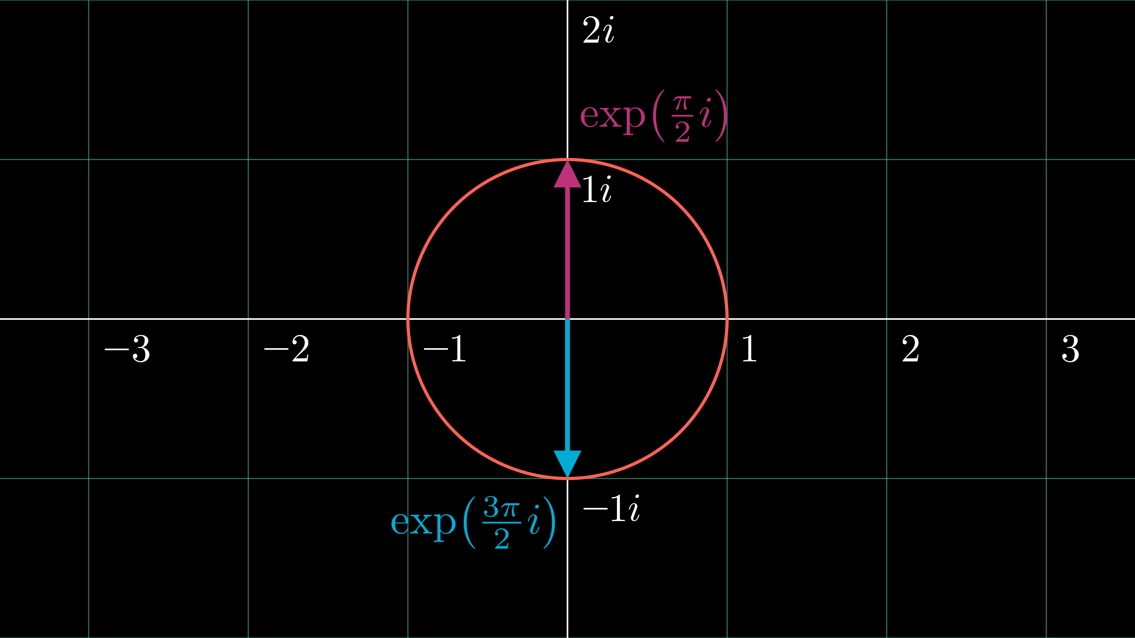

Since this restriction would cause $F_{hkl}$ to collapse to the $y$-axis in the complex plane, it would lead to $\phi_{hkl} = \tfrac{\pi}{2}$ or $\tfrac{3\pi}{2}$. As a final illustrative example, tetragonal space-group symmetry (often observed, for instance, in the enantiomorphic space groups $\text{P}4_{1}2_{1}2$ and $\text{P}4_{3}2_{1}2$) yields the following Argand diagram for certain reflections:

In sum, slightly more complex phase restrictions arise in higher-symmetry space groups! ↩

2. A useful property of any 3D rotation matrix is that its inverse $\textbf{R}^{-1}$ is equivalent to its transpose $\textbf{R}^{T}$. A quick proof of this idea is given in P. R. Evans, Rotations and rotation matrices, Acta Cryst. D57, 1355-1359 (2001). I've written this using $\textbf{R}^{-1}$ because it felt more conceptually satisfying to link the inverse of a rotation matrix with its reciprocal-space counterpart. Nevertheless, since taking the transpose of a $3 \times 3$ matrix is usually much simpler to do on the fly than finding its inverse, feel free to mentally substitute $\textbf{R}^{T}$. ↩

3. This doesn't hold true for 3-fold, 4-fold, or 6-fold rotation matrices, where $\textbf{R} \neq \textbf{R}^{-1}$. ↩